What is correlation in statistics. The correlation coefficient is a characteristic of the correlation model. How to interpret the value of the Pearson correlation coefficient

» Statistics
Statistics and data processing in psychology
(continuation)
Correlation analysis
When studying correlations try to establish whether there is any relationship between two indicators in the same sample (for example, between the height and weight of children or between the level IQ and school performance) or between two different samples (for example, when comparing pairs of twins), and if this relationship exists, whether an increase in one indicator is accompanied by an increase (positive correlation) or a decrease (negative correlation) of the other.
In other words, correlation analysis helps to establish whether it is possible to predict the possible values of one indicator, knowing the value of another.
Until now, when analyzing the results of our experience in studying the effects of marijuana, we have deliberately ignored such an indicator as reaction time. Meanwhile, it would be interesting to check whether there is a relationship between the efficiency of reactions and their speed. This would allow, for example, to argue that the slower a person is, the more accurate and effective his actions will be and vice versa.
To this end, two different methods can be used: the parametric method of calculating the Bravais-Pearson coefficient (r) and the calculation of the Spearman rank correlation coefficient (r s), which is applied to ordinal data, i.e. is non-parametric. However, let's first understand what a correlation coefficient is.
Correlation coefficient
The correlation coefficient is a value that can vary from +1 to -1. In the case of a complete positive correlation, this coefficient is equal to plus 1, and in the case of a complete negative correlation, it is minus 1. On the graph, this corresponds to a straight line passing through the points of intersection of the values of each data pair:
If these points do not line up in a straight line, but form a “cloud”, the absolute value of the correlation coefficient becomes less than one and approaches zero as the cloud rounds off:

If the correlation coefficient is 0, both variables are completely independent of each other.
In the humanities, a correlation is considered strong if its coefficient is greater than 0.60; if it exceeds 0.90, then the correlation is considered very strong. However, in order to be able to draw conclusions about the relationships between variables, the sample size is of great importance: the larger the sample, the more reliable the value of the obtained correlation coefficient. There are tables with critical values of the Bravais-Pearson and Spearman correlation coefficients for a different number of degrees of freedom (it is equal to the number of pairs minus 2, i.e. n- 2). Only if the correlation coefficients are greater than these critical values can they be considered reliable. So, in order for the correlation coefficient of 0.70 to be reliable, at least 8 pairs of data should be taken into the analysis ( h =n-2=6) when calculating r (see Table 4 in the Appendix) and 7 pairs of data (h = n-2= 5) when calculating r s (Table 5 in the Appendix).
I would like to emphasize once again that the essence of these two coefficients is somewhat different. The negative coefficient r indicates that the efficiency is most often the higher, the faster the reaction time, while when calculating the coefficient r s it was necessary to check whether faster subjects always react more accurately, and slower subjects less accurately.
Bravais-Pearson correlation coefficient (r) - This is a parametric indicator, for the calculation of which the average and standard deviations of the results of two measurements are compared. In this case, a formula is used (it may look different for different authors)
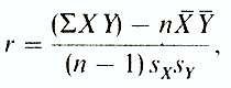
where Σ XY- the sum of the products of the data from each pair;
n is the number of pairs;
X - average for given variable x;
Y -
average for variable data Y
Sx- standard deviation for distribution X;
Sy- standard deviation for distribution at
Spearman rank correlation coefficient ( rs ) - this is a non-parametric indicator, with the help of which they try to reveal the relationship between the ranks of the corresponding quantities in two series of measurements.
This coefficient is easier to calculate, but the results are less accurate than using r. This is due to the fact that when calculating the Spearman coefficient, the order of the data is used, and not their quantitative characteristics and intervals between classes.
The fact is that when using the correlation coefficient of Spearman ranks (r s), they only check whether the ranking of data for any sample will be the same as in a series of other data for this sample, pairwise related to the first (for example, whether they will be the same " ranked” by students in both psychology and mathematics, or even with two different psychology teachers?). If the coefficient is close to +1, then this means that both series practically coincide, and if this coefficient is close to -1, we can talk about a complete inverse relationship.
Coefficient rs calculated according to the formula
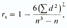
where d is the difference between the ranks of conjugate feature values (regardless of its sign), and is the number of pairs.
Typically, this non-parametric test is used in cases where you need to draw some conclusions not so much about intervals between the data, how much about them ranks, and also when the distribution curves are too skewed and do not allow the use of parametric criteria such as the coefficient r (in these cases it may be necessary to turn quantitative data into ordinal data).
Summary
So, we have considered various parametric and non-parametric statistical methods used in psychology. Our review was very superficial, and its main task was to make the reader understand that statistics are not as scary as they seem, and require mostly common sense. We remind you that the data of "experience" with which we have dealt here are fictitious and cannot serve as a basis for any conclusions. However, such an experiment would be worth doing. Since a purely classical technique was chosen for this experiment, the same statistical analysis could be used in many different experiments. In any case, it seems to us that we have outlined some main directions that may be useful to those who do not know where to start the statistical analysis of the results.
Literature
- Godefroy J. What is psychology. - M., 1992.
- Chatillon G., 1977. Statistique en Sciences humaines, Trois-Rivieres, Ed. SMG.
- Gilbert N. 1978. Statistiques, Montreal, Ed. H.R.W.
- Moroney M.J., 1970. Comprendre la statistique, Verviers, Gerard et Cie.
- Siegel S., 1956. Non-parametric Statistic, New York, MacGraw-Hill Book Co.
Spreadsheet Application
Notes. 1) For large samples or significance levels less than 0.05, refer to tables in statistical textbooks.
2) Tables of values for other non-parametric criteria can be found in special guidelines (see bibliography).
| Table 1. Criterion values t Student | |
| h | 0,05 |
| 1 | 6,31 |
| 2 | 2,92 |
| 3 | 2,35 |
| 4 | 2,13 |
| 5 | 2,02 |
| 6 | 1,94 |
| 7 | 1,90 |
| 8 | 1,86 |
| 9 | 1,83 |
| 10 | 1,81 |
| 11 | 1,80 |
| 12 | 1,78 |
| 13 | 1,77 |
| 14 | 1,76 |
| 15 | 1,75 |
| 16 | 1,75 |
| 17 | 1,74 |
| 18 | 1,73 |
| 19 | 1,73 |
| 20 | 1,73 |
| 21 | 1,72 |
| 22 | 1,72 |
| 23 | 1,71 |
| 24 | 1,71 |
| 25 | 1,71 |
| 26 | 1,71 |
| 27 | 1,70 |
| 28 | 1,70 |
| 29 | 1,70 |
| 30 | 1,70 |
| 40 | 1,68 |
| ¥ | 1,65 |
| Table 2. Values of the criterion χ 2 | |
| h | 0,05 |
| 1 | 3,84 |
| 2 | 5,99 |
| 3 | 7,81 |
| 4 | 9,49 |
| 5 | 11,1 |
| 6 | 12,6 |
| 7 | 14,1 |
| 8 | 15,5 |
| 9 | 16,9 |
| 10 | 18,3 |
| Table 3. Reliable Z values | |
| R | Z |
| 0,05 | 1,64 |
| 0,01 | 2,33 |
| Table 4. Reliable (critical) values of r | ||
| h =(N-2) | p= 0,05 (5%) | |
| 3 | 0,88 | |
| 4 | 0,81 | |
| 5 | 0,75 | |
| 6 | 0,71 | |
| 7 | 0,67 | |
| 8 | 0,63 | |
| 9 | 0,60 | |
| 10 | 0,58 | |
| 11 | 0.55 | |
| 12 | 0,53 | |
| 13 | 0,51 | |
| 14 | 0,50 | |
| 15 | 0,48 | |
| 16 | 0,47 | |
| 17 | 0,46 | |
| 18 | 0,44 | |
| 19 | 0,43 | |
| 20 | 0,42 | |
| Table 5. Reliable (critical) values of r s | |
| h =(N-2) | p = 0,05 |
| 2 | 1,000 |
| 3 | 0,900 |
| 4 | 0,829 |
| 5 | 0,714 |
| 6 | 0,643 |
| 7 | 0,600 |
| 8 | 0,564 |
| 10 | 0,506 |
| 12 | 0,456 |
| 14 | 0,425 |
| 16 | 0,399 |
| 18 | 0,377 |
| 20 | 0,359 |
| 22 | 0,343 |
| 24 | 0,329 |
| 26 | 0,317 |
| 28 | 0,306 |
Correlation coefficient is a value that can vary from +1 to -1. In the case of a complete positive correlation, this coefficient is equal to plus 1 (they say that with an increase in the value of one variable, the value of another variable increases), and with a complete negative correlation - minus 1 (indicate feedback, i.e. When the values of one variable increase, the values of the other decrease).

 Ex 1:
Ex 1:
Dependence graph of shyness and depression. As you can see, the dots (subjects) are not located randomly, but line up around one line, and, looking at this line, we can say that the higher the shyness is expressed in a person, the more depressive, i.e. these phenomena are interconnected.
 Ex 2: Graph for Shyness and Sociability. We see that as shyness increases, sociability decreases. Their correlation coefficient is -0.43. Thus, a correlation coefficient greater from 0 to 1 indicates a directly proportional relationship (the more ... the more ...), and a coefficient from -1 to 0 indicates an inversely proportional relationship (the more ... the less ...)

 If the correlation coefficient is 0, both variables are completely independent of each other.
correlation- this is a relationship where the impact of individual factors appears only as a trend (on average) with the mass observation of actual data. Examples of correlation dependence can be the dependence between the size of the bank's assets and the amount of the bank's profit, the growth of labor productivity and the length of service of employees.
Two systems of classification of correlations according to their strength are used: general and particular.
The general classification of correlations: 1) strong, or close with a correlation coefficient of r> 0.70; 2) medium at 0.500.70, and not just a correlation of a high level of significance.The following table lists the names of the correlation coefficients for different types of scales.
| Dichotomous scale (1/0) | Rank (ordinal) scale | ||
| Dichotomous scale (1/0) | Pearson's association coefficient, Pearson's four-cell conjugation coefficient. | Biserial correlation | |
| Rank (ordinal) scale | Rank-biserial correlation. | Spearman's or Kendall's rank correlation coefficient. | |
| Interval and absolute scale | Biserial correlation | The values of the interval scale are converted into ranks and the rank coefficient is used | Pearson correlation coefficient (linear correlation coefficient) |
At r=0 there is no linear correlation. In this case, the group means of the variables coincide with their general means, and the regression lines are parallel to the coordinate axes.
Equality r=0 speaks only of the absence of a linear correlation dependence (uncorrelated variables), but not in general about the absence of a correlation, and even more so, a statistical dependence.
Sometimes the conclusion that there is no correlation is more important than the presence of a strong correlation. A zero correlation of two variables may indicate that there is no influence of one variable on the other, provided that we trust the results of the measurements.
In SPSS: 11.3.2 Correlation coefficients
Until now, we have found out only the very fact of the existence of a statistical relationship between two features. Next, we will try to find out what conclusions can be drawn about the strength or weakness of this dependence, as well as about its form and direction. Criteria for quantifying the relationship between variables are called correlation coefficients or measures of connectivity. Two variables are positively correlated if there is a direct, unidirectional relationship between them. In a unidirectional relationship, small values of one variable correspond to small values of the other variable, large values correspond to large ones. Two variables are negatively correlated if there is an inverse relationship between them. With a multidirectional relationship, small values of one variable correspond to large values of the other variable and vice versa. The values of the correlation coefficients are always in the range from -1 to +1.
Spearman's coefficient is used as a correlation coefficient between variables belonging to the ordinal scale, and Pearson's correlation coefficient (moment of products) is used for variables belonging to the interval scale. In this case, it should be noted that each dichotomous variable, that is, a variable belonging to the nominal scale and having two categories, can be considered as ordinal.
First, we will check if there is a correlation between the sex and psyche variables from the studium.sav file. In doing so, we take into account that the dichotomous variable sex can be considered an ordinal variable. Do the following:
Select from the command menu Analyze (Analysis) Descriptive Statistics (Descriptive statistics) Crosstabs... (Contingency tables)
· Move the variable sex to a list of rows and the variable psyche to a list of columns.
· Click the Statistics... button. In the Crosstabs: Statistics dialog, check the Correlations box. Confirm your choice with the Continue button.
· In the Crosstabs dialog, stop displaying tables by checking the Supress tables checkbox. Click the OK button.
The Spearman and Pearson correlation coefficients will be calculated, and their significance will be tested:
/ SPSS 10
Task number 10 Correlation analysis
The concept of correlation
Correlation or correlation coefficient is a statistical indicator probabilistic relationships between two variables measured on quantitative scales. In contrast to the functional connection, in which each value of one variable corresponds to strictly defined the value of another variable, probabilistic connection characterized by the fact that each value of one variable corresponds to set of values Another variable, An example of a probabilistic relationship is the relationship between height and weight of people. It is clear that people of different weights can have the same height and vice versa.
Correlation is a value between -1 and + 1 and is denoted by the letter r. Moreover, if the value is closer to 1, then this means the presence of a strong connection, and if it is closer to 0, then a weak one. Correlation value less than 0.2 is considered as weak correlation, more than 0.5 - high. If the correlation coefficient is negative, this means that there is an inverse relationship: the higher the value of one variable, the lower the value of the other.
Depending on the accepted values of the coefficient r, different types of correlation can be distinguished:
Strong positive correlation is determined by the value r=1. The term "strict" means that the value of one variable is uniquely determined by the values of another variable, and the term " positive" - that as the value of one variable increases, the value of the other variable also increases.
Strict correlation is a mathematical abstraction and almost never occurs in real research.
positive correlation corresponds to the values 0
Lack of correlation is determined by the value r=0. A correlation coefficient of zero indicates that the values of the variables are not related to each other in any way.
Lack of correlation H o : 0 r xy =0 formulated as a reflection null hypotheses in correlation analysis.
negative correlation: -1
Strong negative correlation determined by the value r= -1. It, like a strict positive correlation, is an abstraction and does not find expression in practical research.
Table 1
Types of correlation and their definitions
The method of calculating the correlation coefficient depends on the type of scale on which the values of the variable are measured.
Correlation coefficient rPearson is the main one and can be used for variables with nominal and partially ordered interval scales, the distribution of values over which corresponds to normal (correlation of product moments). The Pearson correlation coefficient gives fairly accurate results in cases of abnormal distributions as well.
For distributions that are not normal, it is preferable to use the Spearman and Kendall rank correlation coefficients. They are ranked because the program pre-ranks the correlated variables.
The SPSS program calculates the r-Spearman correlation as follows: first, the variables are converted to ranks, and then the Pearson-formula is applied to the ranks.
The correlation proposed by M. Kendall is based on the idea that the direction of the connection can be judged by comparing the subjects in pairs. If for a pair of subjects the change in X coincides in direction with the change in Y coincides, then this indicates a positive relationship. If it does not match, then about a negative relationship. This coefficient is used mainly by psychologists working with small samples. Since sociologists work with large data arrays, it is difficult to sort through pairs, identify the difference in relative frequencies and inversions of all pairs of subjects in the sample. The most common is the coefficient. Pearson.
Since the correlation coefficient rPearson is the main one and can be used (with some error depending on the type of scale and the level of abnormality in the distribution) for all variables measured on quantitative scales, we will consider examples of its use and compare the results obtained with the results of measurements using other correlation coefficients.
The formula for calculating the coefficient r- Pearson:
r xy = ∑ (Xi-Xav)∙(Yi-Yav) / (N-1)∙σ x ∙σ y ∙
Where: Xi, Yi- Values of two variables;
Xav, Yav - average values of two variables;
σ x , σ y are standard deviations,
N is the number of observations.
Pair correlations
For example, we would like to find out how the answers between different types of traditional values correlate in students' ideas about the ideal place of work (variables: a9.1, a9.3, a9.5, a9.7), and then about the ratio of liberal values (a9 .2, a9.4, a9.6, a9.8). These variables are measured on 5-term ordered scales.
We use the procedure: "Analysis", "Correlations", "Paired". By default, the coefficient Pearson is set in the dialog box. We use the coefficient Pearson
The tested variables are transferred to the selection window: a9.1, a9.3, a9.5, a9.7
By pressing OK, we get the calculation:
Correlations
|
a9.1.t. How important is it to have enough time for family and personal life? |
Pearson correlation |
||||
|
Value(2-sided) |
|||||
|
a9.3.t. How important is it to not be afraid of losing your job? |
Pearson correlation |
||||
|
Value(2-sided) |
|||||
|
a9.5.t. How important is it to have such a boss who will consult with you when making this or that decision? |
Pearson correlation |
||||
|
Value(2-sided) |
|||||
|
a9.7.t. How important is it to work in a well-coordinated team, to feel like a part of it? |
Pearson correlation |
||||
|
Value(2-sided) |
|||||
** Correlation is significant at the 0.01 level (2-sided).
Table of quantitative values of the constructed correlation matrix
Partial correlations:
First, let's build a pairwise correlation between these two variables:
|
Correlations |
|||
|
c8. Feel close to those who live near you, neighbors |
Pearson correlation |
||
|
Value(2-sided) |
|||
|
c12. Feel close to their family |
Pearson correlation |
||
|
Value(2-sided) |
|||
|
**. The correlation is significant at the 0.01 level (2-sided). |
|||
Then we use the procedure for constructing a partial correlation: "Analysis", "Correlations", "Partial".
Suppose that the value “It is important to independently determine and change the order of your work” in relation to the indicated variables will be the decisive factor, under the influence of which the previously identified relationship will disappear or turn out to be of little significance.
|
Correlations |
||||
|
Excluded variables |
c8. Feel close to those who live near you, neighbors |
c12. Feel close to their family |
||
|
c16. Feel close to people who have the same wealth as you |
c8. Feel close to those who live near you, neighbors |
Correlation |
||
|
Significance (2-sided) |
||||
|
c12. Feel close to their family |
Correlation |
|||
|
Significance (2-sided) |
||||
As can be seen from the table, under the influence of the control variable, the relationship decreased slightly: from 0.120 to 0.102. it remains sufficiently high and allows one to disprove the null hypothesis with zero error.
Correlation coefficient
The most accurate way to determine the tightness and nature of the correlation is to find the correlation coefficient. The correlation coefficient is a number determined by the formula:


where r xy is the correlation coefficient;
x i -values of the first feature;
i -values of the second feature;
Arithmetic mean of the values of the first feature
Arithmetic mean of the values of the second feature
To use formula (32), we construct a table that will provide the necessary sequence in the preparation of numbers to find the numerator and denominator of the correlation coefficient.
As can be seen from formula (32), the sequence of actions is as follows: we find the arithmetic means of both signs x and y, we find the difference between the values of the sign and its average (х i - ) and y i - ), then we find their product (х i - ) ( y i - ) – the sum of the latter gives the numerator of the correlation coefficient. To find its denominator, one should square the differences (x i -) and (y i -), find their sums and extract the square root from their product.
So for example 31, finding the correlation coefficient in accordance with formula (32) can be represented as follows (Table 50).
The resulting number of the correlation coefficient makes it possible to establish the presence, closeness and nature of the relationship.
1. If the correlation coefficient is zero, there is no relationship between the features.
2. If the correlation coefficient is equal to one, the relationship between the features is so great that it turns into a functional one.
3. The absolute value of the correlation coefficient does not go beyond the interval from zero to one:
This makes it possible to focus on the tightness of the connection: the closer the coefficient is to zero, the weaker the connection, and the closer to unity, the closer the connection.
4. The sign of the correlation coefficient "plus" means direct correlation, the sign "minus" means the opposite.
Table 50
| x i | i | (х i - ) | (y i - ) | (x i - )(y i - ) | (х i - )2 | (y i - )2 |
| 14,00 | 12,10 | -1,70 | -2,30 | +3,91 | 2,89 | 5,29 |
| 14,20 | 13,80 | -1,50 | -0,60 | +0,90 | 2,25 | 0,36 |
| 14,90 | 14,20 | -0,80 | -0,20 | +0,16 | 0,64 | 0,04 |
| 15,40 | 13,00 | -0,30 | -1,40 | +0,42 | 0,09 | 1,96 |
| 16,00 | 14,60 | +0,30 | +0,20 | +0,06 | 0,09 | 0,04 |
| 17,20 | 15,90 | +1,50 | +2,25 | 2,25 | ||
| 18,10 | 17,40 | +2,40 | +2,00 | +4,80 | 5,76 | 4,00 |
| 109,80 | 101,00 | 12,50 | 13,97 | 13,94 |


Thus, the correlation coefficient calculated in Example 31 is r xy = +0.9. allows us to draw the following conclusions: there is a correlation between the magnitude of the muscle strength of the right and left hands in the studied schoolchildren (the coefficient r xy \u003d + 0.9 is non-zero), the relationship is very close (the coefficient r xy \u003d + 0.9 is close to unity), the correlation is direct (the coefficient r xy = +0.9 is positive), i.e. with an increase in the muscle strength of one of the hands, the strength of the other hand increases.
When calculating the correlation coefficient and using its properties, it should be taken into account that the conclusions give correct results when the features are normally distributed and when the relationship between a large number of values of both features is considered.
In the considered example 31, only 7 values of both features were analyzed, which, of course, is not enough for such studies. We remind here again that the examples, in this book in general and in this chapter in particular, are in the nature of illustrating methods, and not a detailed presentation of any scientific experiments. As a result, a small number of feature values are considered, measurements are rounded - all this is done in order not to obscure the idea of the method with cumbersome calculations.
Particular attention should be paid to the essence of the relationship under consideration. The correlation coefficient cannot lead to the correct results of the study if the analysis of the relationship between the features is carried out formally. Let's go back to example 31. Both considered signs were the values of the muscle strength of the right and left hands. Let's imagine that by feature x i in example 31 (14.0; 14.2; 14.9... ...18.1) we mean the length of randomly caught fish in centimeters, and by feature y i (12.1 ; 13.8; 14.2 ... ... 17.4) - the weight of instruments in the laboratory in kilograms. Formally, using the apparatus of calculations to find the correlation coefficient and in this case also obtaining r xy =+0>9, we should have concluded that there is a close relationship of a direct nature between the length of the fish and the weight of the instruments. The absurdity of such a conclusion is obvious.
To avoid a formal approach to using the correlation coefficient, one should use any other method - mathematical, logical, experimental, theoretical - to identify the possibility of a correlation between signs, that is, to detect the organic unity of signs. Only then can one begin to use correlation analysis and establish the magnitude and nature of the relationship.
In mathematical statistics, there is also the concept multiple correlation- Relationships between three or more features. In these cases, a multiple correlation coefficient is used, consisting of the pairwise correlation coefficients described above.
For example, the correlation coefficient of three signs - x і , y і , z і - is:
where R xyz -multiple correlation coefficient expressing how feature x i depends on features y i and z i ;
r xy -correlation coefficient between features x i and y i ;
r xz - correlation coefficient between features Xi and Zi;
r yz - correlation coefficient between features y i , z i
Correlation analysis is:
Correlation analysisCorrelation- statistical relationship of two or more random variables (or variables that can be considered as such with some acceptable degree of accuracy). At the same time, changes in one or more of these quantities lead to a systematic change in the other or other quantities. The correlation coefficient serves as a mathematical measure of the correlation of two random variables.
Correlation can be positive and negative (it is also possible that there is no statistical relationship - for example, for independent random variables). negative correlation - correlation, in which an increase in one variable is associated with a decrease in another variable, while the correlation coefficient is negative. positive correlation - a correlation in which an increase in one variable is associated with an increase in another variable, while the correlation coefficient is positive.
autocorrelation - statistical relationship between random variables from the same series, but taken with a shift, for example, for a random process - with a shift in time.
The method of processing statistical data, which consists in studying the coefficients (correlations) between variables, is called correlation analysis.
Correlation coefficient
Correlation coefficient or pair correlation coefficient in probability theory and statistics, this is an indicator of the nature of the change in two random variables. The correlation coefficient is denoted by the Latin letter R and can take values between -1 and +1. If the modulo value is closer to 1, then this means the presence of a strong connection (with a correlation coefficient equal to one, they speak of a functional connection), and if closer to 0, then a weak one.
Pearson correlation coefficient
For metric quantities, the Pearson correlation coefficient is used, the exact formula of which was introduced by Francis Galton:
Let X,Y- two random variables defined on the same probability space. Then their correlation coefficient is given by the formula:

 ,
,
where cov is the covariance and D is the variance, or equivalently,
,where the symbol denotes the mathematical expectation.
To graphically represent such a relationship, you can use a rectangular coordinate system with axes that correspond to both variables. Each pair of values is marked with a specific symbol. Such a plot is called a "scatterplot".
The method of calculating the correlation coefficient depends on the type of scale to which the variables refer. So, to measure variables with interval and quantitative scales, it is necessary to use the Pearson correlation coefficient (correlation of product moments). If at least one of the two variables has an ordinal scale, or is not normally distributed, Spearman's rank correlation or Kendal's τ (tau) must be used. In the case when one of the two variables is dichotomous, a point two-series correlation is used, and if both variables are dichotomous, a four-field correlation is used. The calculation of the correlation coefficient between two non-dichotomous variables makes sense only if the relationship between them is linear (unidirectional).
Kendell correlation coefficient
Used to measure mutual disorder.
Spearman's correlation coefficient
Properties of the correlation coefficient
- Cauchy - Bunyakovsky inequality:
Correlation analysis
Correlation analysis- method of processing statistical data, which consists in studying the coefficients ( correlations) between variables. In this case, the correlation coefficients between one pair or multiple pairs of features are compared to establish statistical relationships between them.
Target correlation analysis- provide some information about one variable with the help of another variable. In cases where it is possible to achieve the goal, we say that the variables correlate. In its most general form, the adoption of the hypothesis of the presence of a correlation means that a change in the value of variable A will occur simultaneously with a proportional change in the value of B: if both variables increase, then correlation is positive if one variable increases and the other decreases, correlation is negative.
The correlation reflects only the linear dependence of the quantities, but does not reflect their functional connectivity. For example, if we calculate the correlation coefficient between the values A = sin(x) and B = cos(x), then it will be close to zero, i.e., there is no dependence between the quantities. Meanwhile, the quantities A and B are obviously related functionally according to the law sin 2(x) + cos 2(x) = 1.
Limitations of correlation analysis

 Plots of distributions of pairs (x,y) with corresponding x and y correlation coefficients for each of them. Note that the correlation coefficient reflects a linear relationship (top row), but does not describe a relationship curve (middle row), and is not at all suitable for describing complex, non-linear relationships (bottom row).
 - Application is possible if there are a sufficient number of cases to study: for a particular type of correlation coefficient, it ranges from 25 to 100 pairs of observations.
- The second limitation follows from the hypothesis of correlation analysis, which includes linear dependence of variables. In many cases, when it is reliably known that the dependence exists, the correlation analysis may not give results simply because the dependence is non-linear (expressed, for example, as a parabola).
- By itself, the fact of correlation does not give grounds to assert which of the variables precedes or causes changes, or that the variables are generally causally related to each other, for example, due to the action of a third factor.
Application area
This method of processing statistical data is very popular in economics and social sciences (in particular, in psychology and sociology), although the scope of application of correlation coefficients is extensive: quality control of industrial products, metallurgy, agricultural chemistry, hydrobiology, biometrics, and others.
The popularity of the method is due to two points: the correlation coefficients are relatively easy to calculate, their application does not require special mathematical training. Combined with the ease of interpretation, the ease of application of the coefficient has led to its widespread use in the field of statistical data analysis.
spurious correlation
The often tempting simplicity of a correlation study encourages the researcher to draw false intuitive conclusions about the presence of a causal relationship between pairs of traits, while the correlation coefficients establish only statistical relationships.
In the modern quantitative methodology of the social sciences, in fact, there has been a abandonment of attempts to establish causal relationships between observed variables by empirical methods. Therefore, when researchers in the social sciences talk about establishing relationships between the variables they study, either a general theoretical assumption or a statistical dependence is implied.
see also
- Autocorrelation function
- Cross-correlation function
- covariance
- Determination coefficient
- Regression analysis
Wikimedia Foundation. 2010.
Various features may be related.
There are 2 types of connection between them:
- functional;
- correlation.
Correlation translated into Russian - nothing more than a connection.
In the case of a correlation, there is a correspondence of several values of one attribute to several values of another attribute. As examples, we can consider the established correlations between:
- the length of the paws, neck, beak in birds such as herons, cranes, storks;
- indicators of body temperature and heart rate.
For most biomedical processes, the presence of this type of connection has been statistically proven.
Statistical methods make it possible to establish the fact of the existence of the interdependence of features. The use of special calculations for this leads to the establishment of correlation coefficients (measures of connectivity).
Such calculations are called correlation analysis. It is carried out to confirm the dependence of 2 variables (random variables) on each other, which is expressed by the correlation coefficient.
Using the correlation method allows us to solve several problems:
- identify the relationship between the analyzed parameters;
- knowledge of the presence of a correlation allows solving forecasting problems. Thus, there is a real possibility to predict the behavior of a parameter based on the analysis of the behavior of another correlated parameter;
- classification based on the selection of features independent of each other.
For variables:
- related to the ordinal scale, the Spearman coefficient is calculated;
- related to the interval scale - the Pearson coefficient.
These are the most commonly used parameters, but there are others.
The value of the coefficient can be expressed both positive and negative.
In the first case, with an increase in the value of one variable, an increase in the second is observed. With a negative coefficient, the pattern is reversed.
What is the correlation coefficient for?
Random variables connected with each other can have a completely different nature of this connection. It will not necessarily be functional, the case when there is a direct relationship between the quantities. Most often, both quantities are affected by a whole set of various factors, in cases where they are common to both quantities, the formation of related patterns is observed.
This means that the statistically proven fact of the existence of a relationship between the quantities is not a confirmation that the cause of the observed changes has been established. As a rule, the researcher concludes that there are two interrelated consequences.
Properties of the correlation coefficient
 This statistic has the following properties:
- coefficient value ranges from -1 to +1. The closer to the extreme values, the stronger the positive or negative relationship between the linear parameters. In the case of a zero value, we are talking about the absence of correlation between features;
- a positive value of the coefficient indicates that in the case of an increase in the value of one attribute, an increase in the second is observed (positive correlation);
- negative value - in the case of an increase in the value of one attribute, a decrease in the second is observed (negative correlation);
- approaching the value of the indicator to the extreme points (either -1 or +1) indicates the presence of a very strong linear relationship;
- trait indicators can change with a constant value of the coefficient;
- the correlation coefficient is a dimensionless quantity;
- the presence of a correlation is not a mandatory confirmation of a causal relationship.
Correlation coefficient values
The strength of the correlation can be characterized by resorting to the Cheldok scale, in which a qualitative characteristic corresponds to a certain numerical value.
 In case of positive correlation at value:
- 0-0.3 - correlation is very weak;
- 0.3-0.5 - weak;
- 0.5-0.7 - medium strength;
- 0.7-0.9 - high;
- 0.9-1 - very high correlation strength.
The scale can also be used for negative correlation. In this case, the qualitative characteristics are replaced by opposite ones.
You can use the simplified Cheldok scale, in which only 3 gradations of the strength of the correlation are distinguished:
- very strong - indicators ± 0.7 - ± 1;
- average - indicators ± 0.3 - ± 0.699;
- very weak - indicators 0 - ± 0.299.
This statistical indicator allows not only to test the assumption of the existence of a linear relationship between the features, but also to establish its strength.
Types of correlation coefficient
Correlation coefficients can be classified by sign and value:
- positive;
- null;
- negative.
Depending on the analyzed values, the coefficient is calculated:
- Pearson;
- Spearman;
- Kendala;
- Fechner signs;
- concordance or multiple rank correlation.
 The Pearson correlation coefficient is used to establish direct links between the absolute values of variables. In this case, the distributions of both series of variables should approach normal. The variables being compared should differ by the same number of varying features. The scale representing the variables must be either an interval scale or a ratio scale.
- precise establishment of correlation strength;
- comparison of quantitative characteristics.
There are few disadvantages of using Pearson's linear correlation coefficient:
- the method is unstable in case of outliers of numerical values;
- using this method, it is possible to determine the correlation strength only for a linear relationship; for other types of mutual relationships of variables, regression analysis methods should be used.
Rank correlation is determined by the Spearman method, which makes it possible to statistically study the relationship between phenomena. Thanks to this coefficient, the actual degree of parallelism of the two quantitatively expressed series of features is calculated, and the closeness of the identified relationship is also estimated.
- not requiring an exact definition of the value of the correlation strength;
- compared indicators have both quantitative and attributive values;
- comparison of rows of features with open variants of values.
Spearman's method refers to non-parametric analysis methods, so there is no need to check the normality of the feature distribution. In addition, it allows you to compare indicators expressed in different scales. For example, comparing the values of the number of red blood cells in a certain volume of blood (continuous scale) and expert assessment, expressed in points (ordinal scale).
The efficiency of the method is negatively affected by a large difference between the values of the compared values. The method is also ineffective in cases where the measured value is characterized by an uneven distribution of values.
Step by step calculation of correlation coefficient in Excel
The calculation of the correlation coefficient involves the sequential execution of a number of mathematical operations.
The above formula for calculating the Pearson coefficient shows how laborious this process is if done manually.
Using the capabilities of Excell speeds up the process of finding the coefficient at times.
It is enough to follow a simple algorithm of actions:
- introduction of basic information - a column of x values and a column of y values;
- in the tools, the Formulas tab is selected and opened;
- in the tab that opens, select "Insert fx function";
- in the dialog box that opens, the statistical function "Correl" is selected, which allows you to calculate the correlation coefficient between 2 data arrays;
- data is entered in the window that opens: array 1 - the range of values of the x column (the data must be selected), array 2 - the range of values of the y column;
- the “OK” key is pressed, the result of calculating the coefficient appears in the “value” line;
- conclusion regarding the presence of a correlation between the 2 data sets and its strength.
A correlation model (CM) is a calculation program that provides a mathematical equation in which the resulting indicator is quantified depending on one or more indicators.
yx \u003d ao + a1x1
where: y - performance indicator, depending on the factor x;
x - factor sign;
a1 - parameter KM, showing how much the effective indicator y will change when the factor x changes by one, if at the same time all other factors affecting y remain unchanged;
ao - parameter KM, which shows the influence of all other factors on the effective indicator y, except for the factor sign x
When choosing the effective and factor indicators of the model, it is necessary to take into account the fact that the effective indicator in the chain of cause-and-effect relationships is at a higher level than the factor indicators.
Characteristics of the correlation model
After calculating the parameters of the correlation model, the correlation coefficient is calculated.
p - pair correlation coefficient, -1 ≤ p ≤ 1, shows the strength and direction of the influence of the factor indicator on the effective one. The closer to 1, the stronger the relationship, the closer to 0, the weaker the relationship. If the correlation coefficient is positive, then the relationship is direct; if it is negative, it is inverse.
Correlation coefficient formula: pxy \u003d (xy-x * 1 / y) / eh * ey
ex=xx2-(x)2 ; eu=y2-(y)2
If the CM is linear multifactorial, having the form:
yx \u003d ao + a1x1 + a2x2 + ... + axp
then a multiple correlation coefficient is calculated for it.
0 ≤ Р ≤ 1 and shows the strength of the influence of all factor indicators taken together on the effective one.
P \u003d 1- ((uh-uy) 2 / (yi - usr) 2)
Where: uh - effective indicator - calculated value;
ui - actual value;
usr - actual value, average.
The calculated value yx is obtained as a result of substitution into the correlation model instead of x1, x2, etc. their actual values.
For single-factor and multi-factor nonlinear models, the correlation ratio is calculated:
1 ≤ m ≤ 1;
It is believed that the relationship between the effective and factor indicators included in the model is weak if the value of the coefficient of closeness of connection (m) is within 0-0.3; if 0.3-0.7 - the tightness of the connection is average; above 0.7-1 - the connection is strong.
Since the correlation coefficient (paired) p, the correlation coefficient (multiple) P, the correlation ratio m are probabilistic values, then their significance coefficients are calculated for them (determined from the tables). If these coefficients are greater than their tabular value, then the coefficients of closeness of connection are significant reasons. If the coefficients of significance of the tightness of the connection are less than the tabular values, or if the coefficient of connection itself is less than 0.7, then not all factor indicators that significantly affect the result are included in the model.
The coefficient of determination clearly demonstrates the percentage of factor indicators included in the model that determine the formation of the result.
If the coefficient of determination is greater than 50, then the model adequately describes the process under study, if it is less than 50, then it is necessary to return to the first stage of construction and revise the selection of factor indicators for inclusion in the model.
Fisher's coefficient or Fisher's criterion characterizes the effectiveness of the model as a whole. If the calculated value of the coefficient exceeds the table value, then the constructed model is suitable for analysis, as well as planning indicators, calculations for the future. Approximate tabular value \u003d 1.5. If the calculated value is less than the table value, it is necessary to build the model first, including the factors that significantly affect the result. In addition to the effectiveness of the model as a whole, each regression coefficient affects the materiality. If the calculated value of this coefficient exceeded the tabular value, then the regression coefficient will be significant, if it is less, then the factor indicator for which this coefficient is calculated is removed from the sample, the calculations start over, but without this factor.
The correlation coefficient is the degree of association between two variables. Its calculation gives an idea of whether there is a relationship between two data sets. Unlike regression, correlation does not allow predicting values. However, the calculation of the coefficient is an important step in the preliminary statistical analysis. For example, we found that the correlation coefficient between the level of foreign direct investment and GDP growth is high. This gives us an idea that in order to ensure prosperity, it is necessary to create a favorable climate specifically for foreign entrepreneurs. Not so obvious conclusion at first glance!
Correlation and causality
Perhaps there is not a single area of statistics that would be so firmly established in our lives. The correlation coefficient is used in all areas of public knowledge. Its main danger lies in the fact that often its high values are speculated in order to convince people and make them believe in some conclusions. However, in fact, a strong correlation does not at all indicate a causal relationship between the quantities.

Correlation coefficient: Pearson and Spearman formula
There are several main indicators that characterize the relationship between two variables. Historically, the first is Pearson's linear correlation coefficient. It is passed at school. It was developed by K. Pearson and J. Yule based on the work of Fr. Galton. This coefficient allows you to see the relationship between rational numbers that change rationally. It is always greater than -1 and less than 1. A negative number indicates an inversely proportional relationship. If the coefficient is zero, then there is no relationship between the variables. Equal to a positive number - there is a directly proportional relationship between the studied quantities. Spearman's rank correlation coefficient makes it possible to simplify calculations by constructing a hierarchy of variable values.

Relationships between variables
Correlation helps answer two questions. First, whether the relationship between variables is positive or negative. Secondly, how strong is the addiction. Correlation analysis is a powerful tool with which to obtain this important information. It is easy to see that household incomes and expenses rise and fall proportionately. Such a relationship is considered positive. On the contrary, when the price of a product rises, the demand for it falls. Such a relationship is called negative. The values of the correlation coefficient are between -1 and 1. Zero means that there is no relationship between the studied values. The closer the indicator to the extreme values, the stronger the relationship (negative or positive). The absence of dependence is evidenced by a coefficient from -0.1 to 0.1. It must be understood that such a value only indicates the absence of a linear relationship.

Application features
The use of both indicators is subject to certain assumptions. First, the presence of a strong relationship does not determine the fact that one value determines the other. There may well be a third quantity that defines each of them. Secondly, a high Pearson correlation coefficient does not indicate a causal relationship between the studied variables. Thirdly, it shows an exclusively linear relationship. Correlation can be used to evaluate meaningful quantitative data (eg barometric pressure, air temperature) rather than categories such as gender or favorite color.
Multiple correlation coefficient
Pearson and Spearman investigated the relationship between two variables. But what to do if there are three or even more of them. This is where the multiple correlation coefficient comes in. For example, the gross national product is affected not only by foreign direct investment, but also by the monetary and fiscal policies of the state, as well as the level of exports. The growth rate and the volume of GDP are the result of the interaction of a number of factors. However, it should be understood that the multiple correlation model is based on a number of simplifications and assumptions. First, multicollinearity between quantities is excluded. Second, the relationship between the dependent variable and the variables that affect it is assumed to be linear.

Areas of use of correlation and regression analysis
This method of finding the relationship between quantities is widely used in statistics. It is most often resorted to in three main cases:
- For testing causal relationships between the values of two variables. As a result, the researcher hopes to find a linear relationship and derive a formula that describes these relationships between quantities. Their units of measurement may be different.
- To check for a relationship between values. In this case, no one determines which variable is dependent. It may turn out that the value of both quantities determines some other factor.
- To derive an equation. In this case, you can simply substitute numbers into it and find out the values of the unknown variable.
A man in search of a causal relationship
Consciousness is arranged in such a way that we definitely need to explain the events that occur around. A person is always looking for a connection between the picture of the world in which he lives and the information he receives. Often the brain creates order out of chaos. He can easily see a causal relationship where there is none. Scientists have to specifically learn to overcome this trend. The ability to evaluate relationships between data is objectively essential in an academic career.
Media bias
Consider how the presence of a correlation can be misinterpreted. A group of ill-behaved British students were asked if their parents smoked. Then the test was published in the newspaper. The result showed a strong correlation between parents' smoking and their children's delinquency. The professor who conducted this study even suggested putting a warning about this on cigarette packs. However, there are a number of problems with this conclusion. First, the correlation does not indicate which of the quantities is independent. Therefore, it is quite possible to assume that the pernicious habit of parents is caused by the disobedience of children. Secondly, it is impossible to say with certainty that both problems did not arise due to some third factor. For example, low-income families. It should be noted the emotional aspect of the initial conclusions of the professor who conducted the study. He was an ardent opponent of smoking. Therefore, it is not surprising that he interpreted the results of his study in this way.

conclusions
Misinterpreting correlation as a causal relationship between two variables can lead to embarrassing research errors. The problem is that it lies at the very core of human consciousness. Many marketing tricks are based on this feature. Understanding the difference between causation and correlation allows you to rationally analyze information both in everyday life and in your professional career.